Charles Matthews | Constrained Molecular Dynamics

Molecular dynamics (MD) is a widely used and powerful tool for studying molecular systems with extensive applications to the simulation of macromolecules both for fundamental biology/biochemistry and, increasingly, for medical applications. In MD simulation of complex systems, the most important restriction (ignoring issues of force field quality) is the size of the timestep that can be used to accurately compute trajectories. The goal of simulation is typically to unlock behaviours that occur on timescales of microseconds or more, for example state-to-state protein conformational dynamics such as partial folds of proteins, but the use of typical MD methods limits the timestep to a few femtoseconds.

The limits on the timestep are typically related to the fastest degrees of freedom in the model, so the method of constraints consists of introducing algebraic relations to freeze selected high-frequency bond lengths and/or bond angles. The use of constraints can enable an increase in the simulation timestep for organic molecules in detailed solvent to between 2 and 4 fs, a substantial improvement on the 1–2 fs typically used for fully flexible models.

The Langevin dynamics equations incorporating holonomic constraints look like the following:

\[\begin{aligned} \mathrm{d} q &= M^{-1}p \,\mathrm{d} t\\ \mathrm{d} p &= -\nabla V(q) \,\mathrm{d} t - \gamma p \,\mathrm{d} t + \sigma\,\mathrm{d}W_t - \lambda \nabla g(q)\\ g(q) &= 0\\\nabla g(q) \cdot M^{-1} p &= 0 \end{aligned}\]

where \(q\) is position, \(p\) is momentum, \(M\) is the diagonal mass matrix, and \(\gamma,\,\sigma\) are positive constants. The constraint itself comes from the \(g\) function, where the solutions all lie on the manifold \(g(q)=0\) (the constraint is holonomic because only the position variables respect it).

The novel method we introduce in the article (called g-BAOAB) solves these equations by splitting them up in to pieces. We can also further split the solvent and solute, and move them forward separately. As the solute part is cheap, we can do multiple iterations per step with minimal cost. We denote the number of inner-solute steps (confusingly) by \(P\).

We test the method on a toy protein (alanine dipeptide, see below) solvated in water.

The toy protein example alanine dipeptide, visualized in VMD (right).

We look at the statistical results for alanine dipeptide with our novel scheme, at timesteps significantly beyond the standard timestep ranges (up to 10fs). In the original article, I added the code to the Tinker package (written in Fortran), but currently the scheme is being developed for the OpenMM package (in Python) instead.

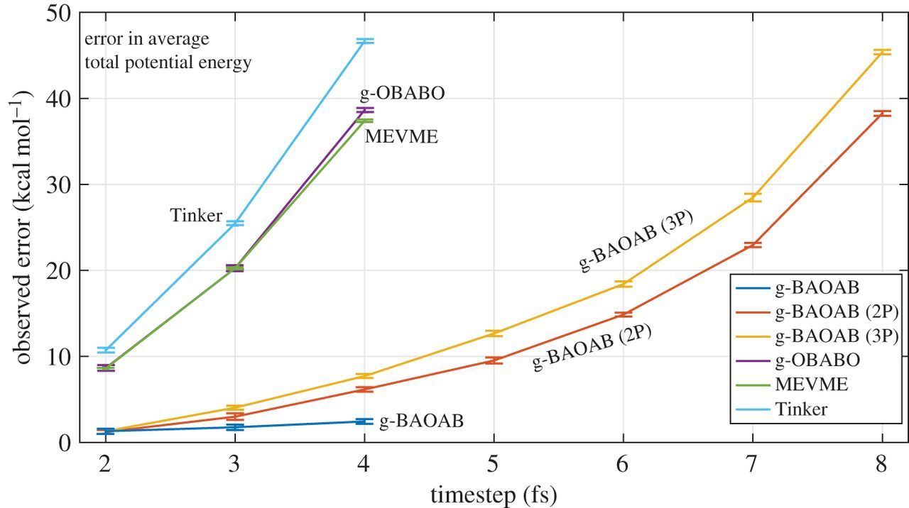
Comparing results for the average potential energy for different methods, as a function of timestep, we can see a clear trend in the Figure below.

The error in average potential energy as a function of timestep, for different methods. Error bars are shown from averaging multiple trajectories.

The g-BAOAB scheme is shown to significantly increase the usable timestep, even when using \(P=1\) where the maximum timestep of 4fs gives minimal error. Using \(P=2\) we obtain a factor of two or three over the standard Tinker scheme and alternative constraint schemes in the literature.

For more details, checkout the article and download the original Tinker add-on code.