Charles Matthews | Cascade failure in power networks

For large-scale electrical power networks, the failure of particular transmission lines can offload power to other lines and cause self-protection trips to activate, instigating a cascade of line failures. In extreme cases, this can bring down the entire network. Learning where the vulnerabilities are and the expected timescales for which failures are likely is an active area of research. This project uses a novel stochastic dynamics model for modelling the dynamics of power networks along with a framework for efficient computer simulation of the model’s development, including long timescale events such as cascade failure. We build on an existing Hamiltonian formulation and introduce stochastic forcing and damping components to simulate small perturbations to the network. Our model and simulation framework allow assessment of the particular weaknesses in a power network that make it susceptible to cascade failure, along with the timescales and mechanism for expected failures.

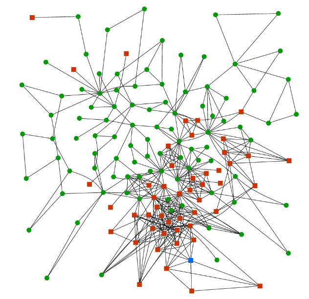
A graphical representation of the benchmark power network used in our tests. There are 145buses (95 load buses as green circles, 49 generators as red squares, and one slack bus as a blue square) connected by 453 power lines.

Our motivation for introducing the stochastic dynamics is to gather statistics and classify failures of the network. The most common way to approximate the behavior of a physical network at a failure point is to mimic the responses of the thermal relay on each power line, by removing a line from service when the energy on the line becomes too large.

We model the failure dynamics as an irreversible change that alters network topology and moves the system’s equilibrium point \(x_\text{eq}\). An interesting feature of our formalism is that we can capture the timescale and trajectory of the system as it transitions between neighborhoods of \(x_\textrm{eq}^{\textrm{(old})}\) to \(x_\textrm{eq}^{\textrm{(new})}\), which correspond to the stable regions before and after a line failure.

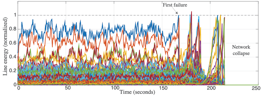
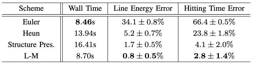
We simulate the dynamics of the power network, with a given threshold at which the line protection activates. After the first failure, the network shortly collapses.

Since the goal of our modeling is to probe the statistics of the system as it evolves, we seek to generate a large number of trajectories by solving the proposed dynamics. Because of the dimensionality of the state \(x\) and the complexity of the Hamiltonian defining the dynamics, finding analytical solutions is not feasible. We turn instead to a numerical timestepping algorithm with time discretization parameter (timestep) \(h >0\) to advance from \(x(t)\) to \(x(t+h)\). The parameter \(h\) is usually chosen after some experimentation – too small a choice increases the computational effort required to simulate to until failure (the hitting time), while increasing \(h\) can create instability in the system or a large error in observed average times.

We look at solving the dynamics using multiple different methods, implemented in a Python package (given below).

The errors using the Hamiltonian formulation with multiple schemes. The L-M method (Leimkuhler-Matthews method) is particularly efficient.

With an accurate numerical method, we experiment with manual disconnection of lines to locate weak points in the network, and using clustering algorithms to qualify the phase changes in the state. We also use the Parallel Replica method (often used in Computational Chemistry) to compute accurate hitting times efficiently. Check out the code and the article for more information.